The modern C++ implementation of the eGFRD has been published as an open source package on GitHub. Please follow the installation instructions on the repository to setup the simulator. Problems can be reported via the eGFRD issue tracker.
Examples
To help you getting started, we have assembled some simple models. These can be used to verify the implementation of the code and to build more complex models.
Equilibrium
Consider a set of particles A, B and C with the following reaction: A + B ⇾ C with binding rate constant ka [m3/s] and C ⇾ A + B and unbinding rate kd [s-1]. In a box with length L [m] and periodic boundary conditions, the reaction will relax towards equilibrium. For this system, we can calculate the number of C particles analytically.
NC_th = { 2•N + KD•V - sqrt[ (2•N + KD•V)2 - 4•N•N ] } / 2
where N is the number of A and B particles respectively in the volume V = L3, and KD = kd/ka is the dissociation constant. To test the eGFRD-simulation a model (equilibrium.gfrd) is provide that sets up this scenario and starts with zero C particles. After some time the number of C particles should approach the calculated equilibrium NC_th. To run this model:
./RunGfrd ../../samples/equilibrium/equilibrium.gfrd
The output of the program shows average amount of particles at intervals of 1 second. The number of C particles should be readily increasing and after reaching equilibrium will fluctuate around the calculated NC_th. Press Ctrl-C to end the simulation.
Now the unbinding rate kd can be changed to a higher value decreasing the average number of C particles in equilibrium. This can be done by editing the model-file in a text-editor or by defining the value kd on the commandline:
./RunGfrd ../../samples/equilibrium/equilibrium.gfrd -d kd=8e-2
Power Spectrum
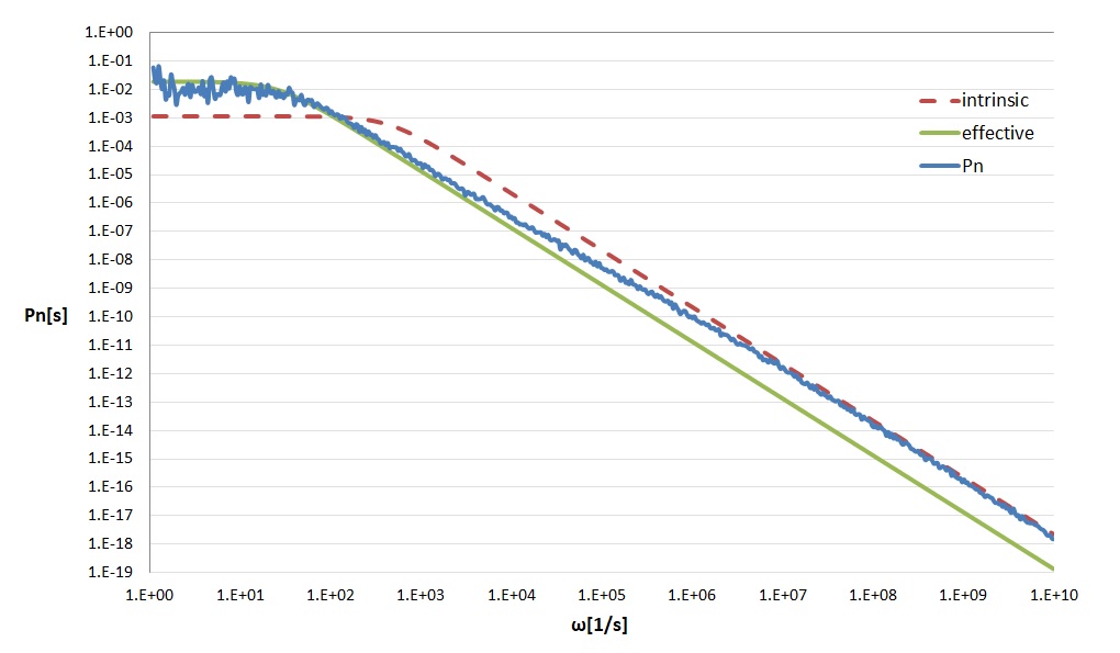
Besides the dissociation constant, it may also prove useful to compute the power spectrum of the simple association-dissociation reaction. The provided model powerspectrum.gfrd sets up the simulator with the same parameters as in the paper of Kaizu et. al. [1]:
./RunGfrd ../../samples/powerspectrum/powerspectrum.gfrd
This simulation writes binding and unbinding event time-stamps in a file ‘power_rec.dat’. A powerspectrum can be calculated from tihs data, e.q. with the provided Python script ‘calcspectrum.py’ or mutch faster the C/C++ code ‘calcspectrum.cpp’. These also calculate the intrinsic and effective curves. See figure below.
MAPK
The Mitogen-Activated Protein Kinase (MAPK) cascade is one of most studied and best characterized signalling pathways in biology. The cascade consists of three layers, where in each layer a protein is phosphorylated at two states. The application of eGFRD to one layer showed that fluctuations at the molecular scale can dramatically change the macroscopic behavior at the cellular scale [2]. With the new eGFRD package the MAPK simulation can be easily set up using:
./RunGfrd ../../samples/mapK/mapK.gfrd
Custom
Users can use the package to set up their own model by creating their a new gfrd-file. This can be from scratch or copy one of the samples as a starting point. See documentation.
.\RunGfrd user-file.gfrd
When the model-language is too restricted or you’re just more confident writing C++ code, it is also possible to do just that. As an staring point the SimCustom.hpp is your place. To start you custom simulator type:
.\RunGfrd --custom
Resume
The simulator (when enabled) writes it’s internal state to a file at every maintanance step (usually the maintanance step is is high number like 100000 or 1000000). In the unfortunate event that something goes wrong (unexpected termination) the state file can be used to resume simulation from the maintanance step before the crash. This is espacially usefull when the simulater fails after days of calculating and you now need to now debug that error.
.\RunGfrd --resume sim_state.dat
Sample model file: rebind.gfrd
; eGFRD rebinding simulation

[Simulator]
           Seed = 0x1234CAFE
        EndTime = 90.0                 ; sec.
MaintenanceStep = 100000
MaintenanceFile = sim_dump.out

[World]
Matrix = 8
  Size = 3.42e-6                      ; 40 femto Liter = 4e-17 m3

[CopyNumbers]
Interval = 1E-1
    File = copy_num.out
    Type = Instantaneous

[SpeciesType]
Name = A B C
   r = 1e-9                            ; m
   D = 1e-12                           ; m^2*s^-1

[ReactionRule]
Rule = A + B <=> C
  ka = 1e-19                           ; m^3*s^-1
  kd = 2e-2                            ; s^-1

[Particles]
A = 100
B = 100
C = 0